Running Pipelines#
Production Studio supports different types of pipelines. The three main pipelines are:
Forward Production Pipeline
Inverse Production Pipeline
Flat Pipeline
Let’s have a look at how to use each of them.
Forward Production Pipeline#
The Forward Production Pipeline simulates future production based on historical data and user-defined parameters.
Define the Parameters for the Forward Simulation
params = {
    "simulation_type": "Forward",
    "num_wells_list": [10, 15, 20],
    "gas_exp_params": [11500, -0.05, 300],
    "oil_exp_params": [23, -0.04, 0.1],
    "num_til_days": 30,
    "simulation_start": "2025-02-01",
    "well_efficiency_factor": 1.2,
    "crew_efficiency_factor": 1.1,
    "well_frac_ratio": 2.5,
}

# Run the forward simulation
forward_results = simulation.run_simulation(params=params)
Output: The following logs will be displayed upon execution.
INFO:Running Forward simulation.
INFO:Simulations request sent with request ID: e6b79e89-1bce-406f-bd9e-4eefbf2c044d.
INFO:Simulation request successful
Visualize the Results
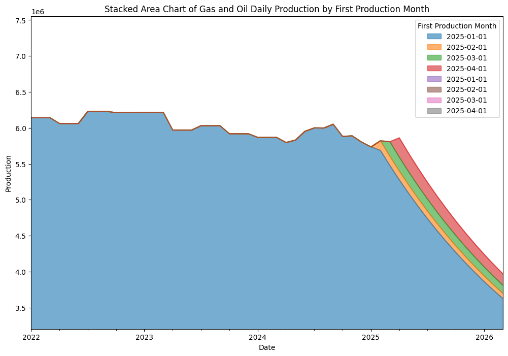
Once the forward simulation has been executed, visualize the results using a stacked area chart of gas and oil daily production over time. The following code can be used to generate the chart.
import matplotlib.pyplot as plt
import pandas as pd

# Extract the user_forecast_df from the results
user_forecast_df = forward_results.user_forecast_df

# Convert the 'date' column to datetime
user_forecast_df['date'] = pd.to_datetime(user_forecast_df['date'])

# Pivot the DataFrame to have 'date' as the index and 'first_production_month' as columns
pivot_df = user_forecast_df.pivot_table(index='date', columns='first_production_month', values=['gas_daily', 'oil_daily'], aggfunc='sum')

# Calculate total production for setting y-axis limits
total_production = pivot_df['gas_daily'].sum(axis=1) + pivot_df['oil_daily'].sum(axis=1)
y_min = 0.8 * total_production.min()
y_max = 1.2 * total_production.max()

# Plot the stacked area chart
fig, ax = plt.subplots(figsize=(12, 8))

# Plot gas_daily
pivot_df['gas_daily'].plot(kind='area', stacked=True, ax=ax, alpha=0.6, title='Gas Daily Production by First Production Month')

# Plot oil_daily
pivot_df['oil_daily'].plot(kind='area', stacked=True, ax=ax, alpha=0.6, title='Oil Daily Production by First Production Month')

# Set labels and title
ax.set_xlabel('Date')
ax.set_ylabel('Production')
ax.set_title('Stacked Area Chart of Gas and Oil Daily Production by First Production Month')

# Set y-axis limits
ax.set_ylim(y_min, y_max)

# Show the legend
ax.legend(title='First Production Month')

# Show the plot
plt.show()
Output: The stacked area chart visualizes daily gas and oil production by first production month, revealing production trends.

Inverse Production Pipeline#
The Inverse Production Pipeline determines the necessary inputs (e.g., number of wells or frac crews) to achieve a target production level.
Define the Parameters for the Inverse Simulation
params = {
    "simulation_type": "Inverse",
    "future_production": [5.85, 5.84, 5.88, 5.9],
    "gas_exp_params": [11500, -0.05, 160],
    "oil_exp_params": [23, -0.04, 0.1],
    "num_til_days": 30,
    "simulation_start": "2025-02-01",
    "well_efficiency_factor": 1.2,
    "crew_efficiency_factor": 1.1,
    "well_frac_ratio": 2.5,
    "production_type": "Gas",
}

# Run the inverse simulation
inverse_results = simulation.run_simulation(params=params)
Output: The following logs will be displayed upon execution.
INFO:Running Inverse simulation.
INFO:Simulations request sent with request ID: 9ac6c93b-8d82-4ba8-8063-692d86a63d6d.
INFO:Simulation request successful
Visualize the Results
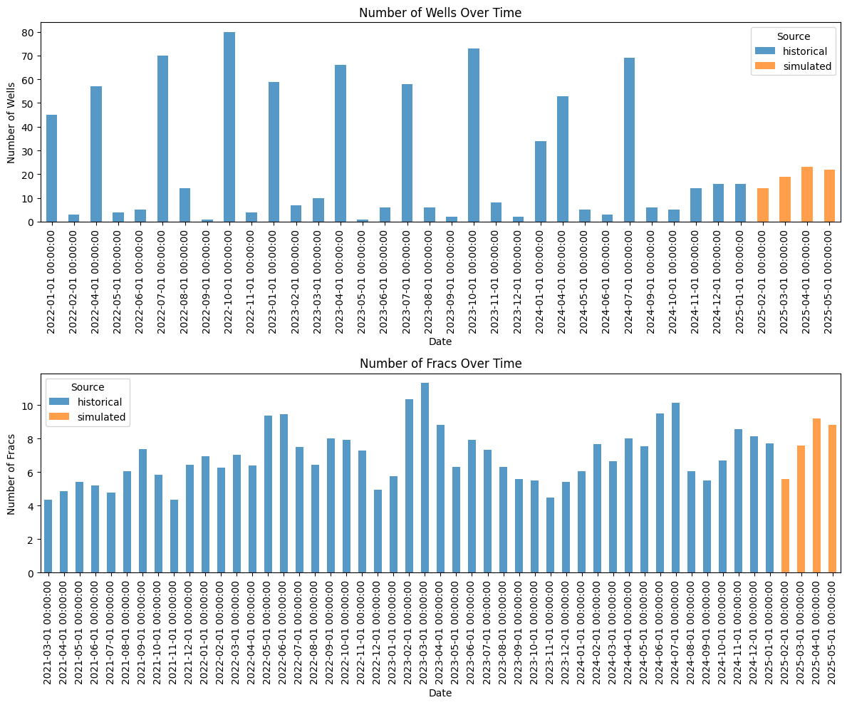
Visualize the results by plotting num_wells_df and num_fracs_df as bar charts. The following code can be used to generate the charts.
# Extract the num_wells_df and num_fracs_df from the results
num_wells_df = inverse_results.num_wells_df
num_fracs_df = inverse_results.num_fracs_df

# Convert the 'date' column to datetime
num_wells_df['date'] = pd.to_datetime(num_wells_df['date'])
num_fracs_df['date'] = pd.to_datetime(num_fracs_df['date'])

# Create subplots
fig, axes = plt.subplots(nrows=2, ncols=1, figsize=(12, 10))

# Plot num_wells_df as a bar chart
num_wells_df.groupby(['date', 'source']).sum()['completions_count'].unstack().plot(kind='bar', stacked=True, ax=axes[0], alpha=0.75)
axes[0].set_title('Number of Wells Over Time')
axes[0].set_xlabel('Date')
axes[0].set_ylabel('Number of Wells')
axes[0].legend(title='Source')

# Plot num_fracs_df as a bar chart
num_fracs_df.groupby(['date', 'source']).sum()['frac_crews_count'].unstack().plot(kind='bar', stacked=True, ax=axes[1], alpha=0.75)
axes[1].set_title('Number of Fracs Over Time')
axes[1].set_xlabel('Date')
axes[1].set_ylabel('Number of Fracs')
axes[1].legend(title='Source')

# Adjust layout
plt.tight_layout()

# Show the plot
plt.show()
Output: The bar charts display the number of wells and frac crews over time.

Flat Simulation Run#
The Flat Production Pipeline determines the necessary inputs (e.g., number of wells of frac crews) to achieve future production equal to recent production level.
Define the Parameters for the Flat Simulation
# Define the parameters for the flat simulation
params = {
    "simulation_type": "Flat",
    "gas_exp_params": [11500, -0.05, 160],
    "oil_exp_params": [23, -0.04, 0.1],
    "num_til_days": 30,
    "simulation_start": "2025-02-01",
    "well_efficiency_factor": 1.2,
    "crew_efficiency_factor": 1.1,
    "well_frac_ratio": 2.5,
    "production_type": "Gas",
    "sim_duration": 12
}

# Run the flat simulation
flat_results = simulation.run_simulation(params=params)
Output: The following logs will be displayed upon execution.
INFO:Running Flat simulation.
INFO:Simulations request sent with request ID: fb1f7210-ca47-4c9c-9b06-76760ca4592d.
INFO:Simulation request successful
Visualize the Results
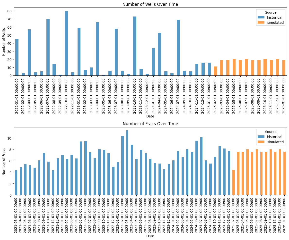
Visualize the results by plotting num_wells_df and num_fracs_df as bar charts. The following code can be used to generate the charts.
# Extract the num_wells_df and num_fracs_df from the results
num_wells_df = flat_results.num_wells_df
num_fracs_df = flat_results.num_fracs_df

# Convert the 'date' column to datetime
num_wells_df['date'] = pd.to_datetime(num_wells_df['date'])
num_fracs_df['date'] = pd.to_datetime(num_fracs_df['date'])

# Create subplots
fig, axes = plt.subplots(nrows=2, ncols=1, figsize=(12, 10))

# Plot num_wells_df as a bar chart
num_wells_df.groupby(['date', 'source']).sum()['completions_count'].unstack().plot(kind='bar', stacked=True, ax=axes[0], alpha=0.75)
axes[0].set_title('Number of Wells Over Time')
axes[0].set_xlabel('Date')
axes[0].set_ylabel('Number of Wells')
axes[0].legend(title='Source')

# Plot num_fracs_df as a bar chart
num_fracs_df.groupby(['date', 'source']).sum()['frac_crews_count'].unstack().plot(kind='bar', stacked=True, ax=axes[1], alpha=0.75)
axes[1].set_title('Number of Fracs Over Time')
axes[1].set_xlabel('Date')
axes[1].set_ylabel('Number of Fracs')
axes[1].legend(title='Source')

# Adjust layout
plt.tight_layout()

# Show the plot
plt.show()

Multiple Forward Simulations#
Multiple Forward Simulations allow users to analyze different production scenarios by running several simulations with varying well and frac parameters.
Define the Parameters for the Multiple Forward Simulation
# Define the parameters for the ForwardSimulation
params = {
    "simulation_type": "ForwardSimulation",
    "num_simulations": 10,
    "well_frac_ranges": [
            {
        "wells_range": [10, 15],
    },
    {
        "wells_range": [10, 20],
    },
    {
        "wells_range": [10, 15],
    },
    {
        "wells_range": [10, 20],
    }
    ],
    "gas_exp_params": [11500, -0.05, 160],
    "oil_exp_params": [23, -0.04, 1],
    "num_til_days": 30,
    "simulation_start": "2025-02-01",
    "well_efficiency_factor": 1.2,
    "crew_efficiency_factor": 1.1,
    "well_frac_ratio": 2.5,
}

# Run the simulation
multi_results = simulation.run_simulation(params)
Output: The following logs will be displayed upon execution.
INFO:Running ForwardSimulation simulation.
INFO:SimulationInputsHandler initialized successfully with duration: 4 months.
INFO:Simulations request sent with request ID: a5bd0424-6fb5-466c-846f-cb427a205fe6.
INFO:Simulation request successful
Randomly Generated Simulation Parameters
The following code retrieves randomly generated simulation parameters for the first simulation.
# Randomly generated simulation parameters for the first simulation
simulation.results['1']['studio_inputs']
Output: The following generated simulation parameters are retrieved for the first simulation.
 {'crew_efficiency_factor': 1.1,
'gas_exp_params': [11500.0, -0.05, 160.0],
'num_fracs_list': [4.0, 6.8, 4.0, 7.2],
'num_months_list': [1, 2, 3, 4],
'num_til_days': 30,
'num_wells_list': [10, 17, 10, 18],
'oil_exp_params': [23.0, -0.04, 1.0],
'simulation_start': '2025-02-01T00:00:00',
'well_efficiency_factor': 1.2,
'well_frac_ratio': 2.5}
Visualize the Results
Visualize the results by plotting a stacked area chart of gas and oil daily production for the first production month. The following code can be used to generate the chart.
import matplotlib.pyplot as plt

def plot_user_forecast_multi_simulation(results):
    """
    Plot the user_forecast_df for each simulation in a multi-simulation as subplots.

    Args:
        results (dict): The dictionary returned by run_multiple_simulations.
    """
    if not isinstance(results, dict):
        print("Results should be a dictionary of simulations.")
        return

    num_simulations = len(results)
    fig, axes = plt.subplots(nrows=num_simulations, ncols=1, figsize=(12, 6 * num_simulations))

    if num_simulations == 1:
        axes = [axes]  # Ensure axes is iterable if there's only one subplot

    for ax, (key, result) in zip(axes, results.items()):
        user_forecast_df = result.user_forecast_df

        # Convert the 'date' column to datetime
        user_forecast_df['date'] = pd.to_datetime(user_forecast_df['date'])

        # Pivot the DataFrame to have 'date' as the index and 'first_production_month' as columns
        pivot_df = user_forecast_df.pivot_table(index='date', columns='first_production_month', values=['gas_daily', 'oil_daily'], aggfunc='sum')

        # Calculate total production for setting y-axis limits
        total_production = pivot_df['gas_daily'].sum(axis=1) + pivot_df['oil_daily'].sum(axis=1)
        y_min = 0.8 * total_production.min()
        y_max = 1.2 * total_production.max()

        # Plot the stacked area chart
        pivot_df['gas_daily'].plot(kind='area', stacked=True, ax=ax, alpha=0.6, title=f'Gas Daily Production by First Production Month - Simulation {key}')
        pivot_df['oil_daily'].plot(kind='area', stacked=True, ax=ax, alpha=0.6, title=f'Oil Daily Production by First Production Month - Simulation {key}')

        # Set labels and title
        ax.set_xlabel('Date')
        ax.set_ylabel('Production')
        ax.set_title(f'Stacked Area Chart of Gas and Oil Daily Production by First Production Month - Simulation {key}')

        # Set y-axis limits
        ax.set_ylim(y_min, y_max)

        # Show the legend
        ax.legend(title='First Production Month')

    # Adjust layout
    plt.tight_layout()

    # Show the plot
    plt.show()

# Example usage
# Assuming 'results' is the dictionary returned by run_multiple_simulations
plot_user_forecast_multi_simulation(multi_results)
